


 167 / 324

In recent times, technological progress allo-
wed more advanced tools to be used, including
in vitro studies with MRI on cadaveric speci-
mens [8, 9], in vivo analyses using 2D fluoro-
scopy with shape matching techniques, based
on CT models [10-13], roentgen stereo photo-
grammetric analysis [14] and open dual coil
MRI’s [15-17]. These newer methods revealed
a more complete, three-dimensional insight in
the morphology and kinematic patterns of the
normal knee in loaded and unloaded condi-
tions. Nevertheless, correct description of knee
kinematics, allowing clinical applications,
remains a major challenge: as Kinzel and
Gutkowski stated, “the unambiguous descrip-
tion of spatial motion is perhaps more difficult
than the measurement” [18].
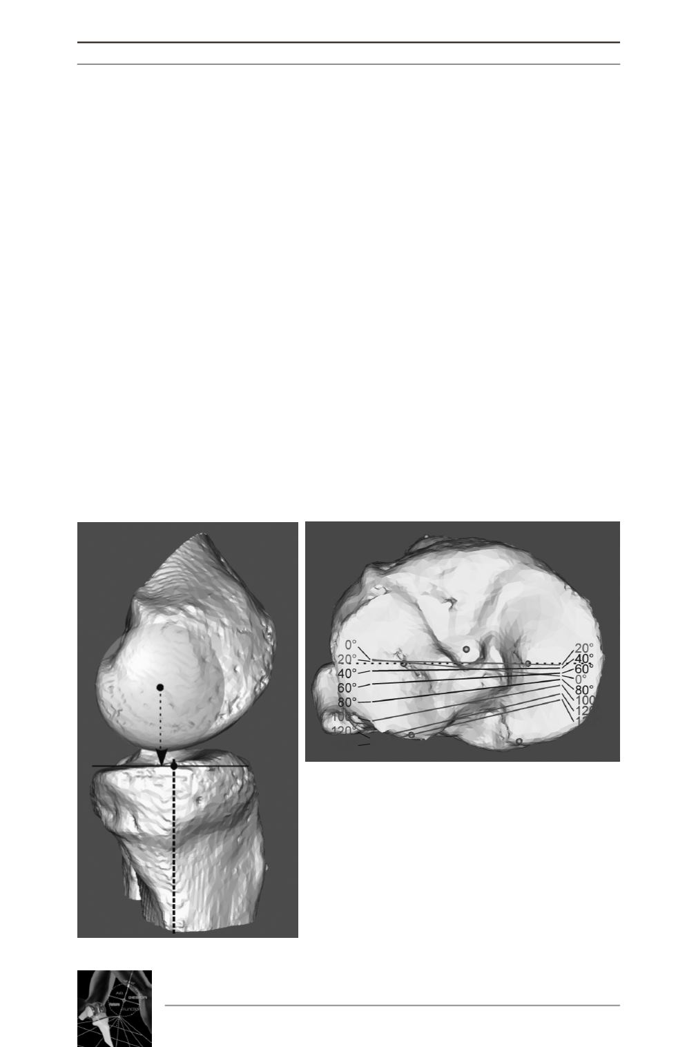
For reasons of practical understanding and cli-
nical application, knee kinematics are current-
ly often presented as the projection of the
centre of the femoral condyles onto the hori-
zontal plane of the tibia, as a function of the
flexion angle (fig. 1).
This presentation of kinematics gives a good
intuitive understanding of the motion between
tibia and femur but it is important to unders-
tand that it is a simplification of a complex
three dimensional motion. Neither is this pre-
sentation identical to the imaging of tibiofe-
moral contact points. The latter technique is
most often used for the description of kinema-
tics after TKA. Based on single perspective
video imaging, a model fitting process allows
to determine the relative three dimensional
position of the implants (fig 2). The presumed
tibiofemoral contact point is derived from a
calculation that determines the shortest distan-
ce between the tibia and the femur.
14
es
JOURNÉES LYONNAISES DE CHIRURGIE DU GENOU
166
Fig. 1 :
a) Projection of the centre of the femoral condyle
onto the horizontal plane of the tibia [19].
b) Lines connecting the projected points as a func-
tion of the flexion angle.
a
b